This post is an overview of my thesis work carried out at the Department of Electrical and Computer Engineering, University of Minnesota-Twin Cities. My thesis work examines a semi-blind source separation problem which finds applications in audio, image, and video processing. The primary aim of this tutorial is to develop an overall intuitive understanding of my work. Suitable examples from our day-to-day lives are employed to motivate and develop the algorithmic framework.

Introduction

If you have ever been to a really noisy party or a large gathering, you must have noticed that you can turn your attention to a specific person and listen to him/her in spite of all the other sounds. It is interesting how you can recognize and keep track of which voice(s) to follow. This process of selective hearing, in signal processing literature, is referred to as the cocktail-party problem or the source separation problem. This problem has been well studied in literature and is of great interest in the signal processing community. However, most of the previous work in this area deals with separating the sources based on either of two simplifying assumptions [[ICA]],

• The sources (speakers) which are inherently independent, meaning they sound very differently to begin with.
• The methods assume that multiple mixtures, equal to the number of individual sources, are available.

In real life situations such independence and availability of these multiple mixtures of the sources are luxuries that we seldom have. For the source separation task we set out to solve at the cocktail-party, the voices of the speakers are somewhat similar, and we say that the sources (voices of individual speakers) are correlated. In addition, because we perform this task (separation of one speaker’s sound from many) on a single recording, this is a single channel source separation task. In this regard, one can view the source separation task as disentangling a mixture of often correlated sources. In cases where none of the sources are known a priori, the problem is known as a Blind Source Separation Problem and when knowledge about some of the sources is available, we refer to it as a Semi-Blind Source Separation Problem.

A Motivating Example in Audio Forensics

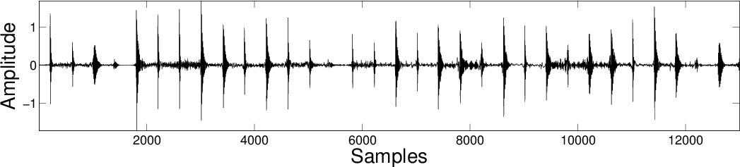
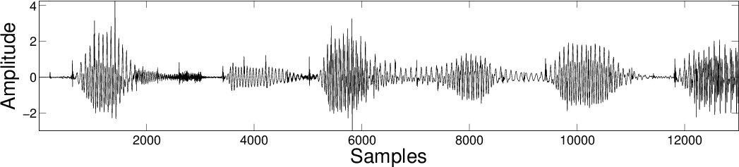
The semi-blind source separation problem studied in this work is motivated from its application in electroshock law enforcement devices. These devices, when fired, eject probes which attach to the suspect and deliver electric current to restrict their movement. A microphone mounted on the gun records the sounds during the event, which is a mixture of ambient noise (people talking/shouting) along with a signal which indicates the status of the device (whether it was delivering current or not). It is often of interest to determine whether the probes were successfully attached and delivering current. However, due to the ambient noise, the fact the two states of the device (delivering and not-delivering current) are highly correlated and other non-idealities, we have a somewhat difficult task at hand.

A visit to the Minnesota Orchestra

After the hostile situation we encountered above, it is time we relax a little by visiting the Minnesota Orchestra. Suppose that you are at the Minnesota Orchestra and after the first act your friends are excitedly discussing about the Cello in the piece you just heard. Now, imagine you have no idea about how the Cello sounds like. What would you do?

You have the following options:

• Case 1: Listen to a sample of a Cello before the next act.
• Case 2: Assuming that you can identify all other instruments, try identifying the Cello and learn what it sounds like during the next act.

These two processes by which you recognize the instrument (Cello) are at the heart of Machine Learning literature. In the cases described above, you either have the training data (Case 1) to learn the instruments or you have the knowledge about all other instruments and you learn the features specific to Cello, on the fly, from the data (Case 2, referred to as an online methodology).

In the situation described above, we often employ the terms like training and learning. Before we delve into the algorithmic specifics of the original problem of semi-blind source separation we set out to solve, let us get introduced to these terms and a new technique available in data analysis and machine learning viz Dictionary Learning.

Dictionary Learning

The word dictionary paints a picture of a resource which contains the meanings of all the words of a language. In an analogous fashion, one can create a dictionary of types of cats, dogs etc., which gives us information about types of cats or dogs respectively. It is assumed that a dictionary of dogs must not be used to look up cats and vice versa. However, it is important to note that both cats and dogs have some features like four feet, two-eyes etc. which are common. In this regard, we note that a good dictionary for a specific class has the distinguishing features of that class i.e. the features that can be used to identify the class.

There is yet another term to be tackled before we describe Dictionary Learning, this is Sparsity. When we say that a signal has a Sparse representation in a dictionary, we mean that that signal can be formed by using a few elements of a specific Dictionary. It is like saying that you have a set of spices and you use a certain (small) number of spices for a specific dish. These individual spices will form the sparse basis for all spice preparations you will use in you meals. All these individual spices hence form the dictionary of spices.

Now, Dictionary Learning is a process by which we aim to learn these distinguishing features of a class from a dataset (known as training data). This technique essentially learns the sparsifying features of a dataset. So why are we interested in sparsifying dictionaries (dictionaries which yield sparse representations)? Sparsifying dictionaries help us to represent the signals succinctly, such compact representations can help us define a particular class efficiently. When such dictionaries are learned on the go, without the use of prior training, it is known as Online Dictionary Learning [[Mairal 2010]].

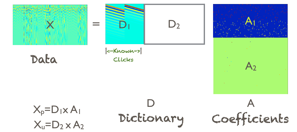
Semi-Blind Morphological Component Analysis

Revisiting the Cellist: the SBMCA Algorithmic framework

We describe the algorithmic motivation to solve the single channel semi-blind source separation problem based on the Online Dictionary Learning technique discussed above by using the technique similar to Case 2 described in Section 3.

Imagine that you have individual dictionaries containing the defining features of each instrument being played at the orchestra except for the Cello. Our essential aim here is to find the part of the musical piece which cannot be represented in these a priori known dictionaries and learn a new dictionary of features describing this unrepresented part (or instrument). This new dictionary (for our example) hence describes the Cello.

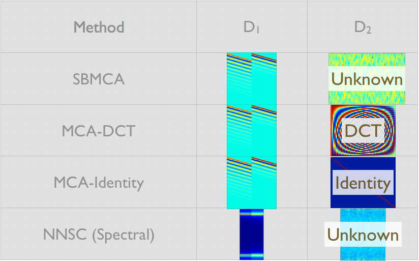
This forms the algorithmic basis of the technique developed to solve the single channel semi-blind source separation problem. More formally, in each iteration of the algorithm we aim to find the representation of a signal in a set of known dictionaries and in the next step learn the unknown dictionary. After a few iterations, we have the desired source separation via their representations in these distinct dictionaries. We call this algorithmic framework as the Semi-Blind Morphological Component Analysis (SBMCA) as it is similar to the Morphological Component Analysis (MCA) [[Starck 2005]], [[Donoho 2010]], [[Bobin 2007]] technique for which all dictionaries are known.

Back to the Audio Forensics Application

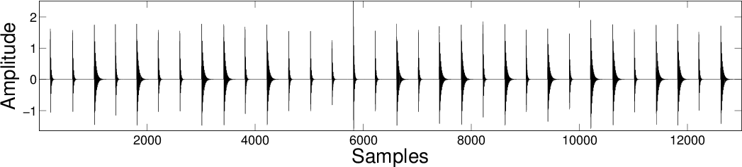
For the Audio Forensics application described in Section 2, we can obtain the information about the delivering and non-delivering current states by triggering the device in a laboratory setting. We form the known dictionaries by using this information about the state signals of the device. In addition, we use the algorithm described above to separate the state signal from the unknown background signal. Subsequently, the state signal can be used to identify the time instants at which the current was being delivered by the electro-shock law enforcement device.

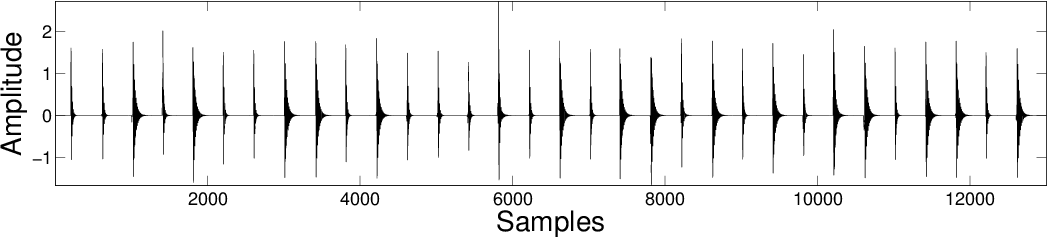
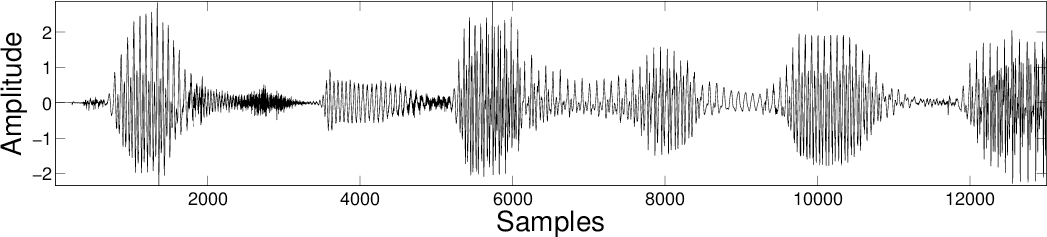
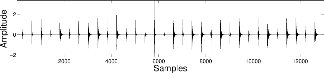
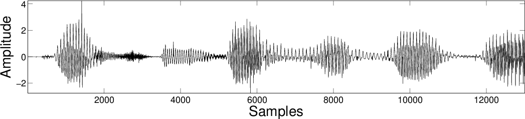
Results

Original Mixture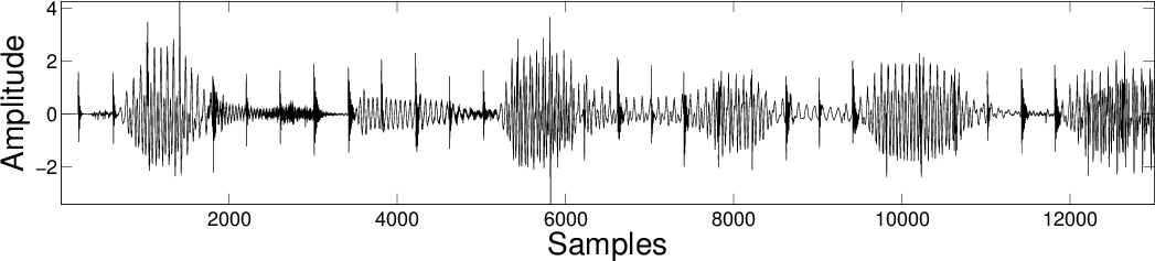
SBMCA
MCA DCT
MCA Identity
NNSC

Conclusions

We motivate and propose a technique to solve the single channel semi-blind source separation problem via Semi-Blind Morphological Component Analysis. We base our discussion on intuition and motivating examples from day to day life. For a deeper analysis, algorithmic details and the results please see [[Rambhatla 2013]].

ICA UMTC Mairal 2010 Starck 2005 Donoho 2010 Bobin 2007 Rambhatla 2013